Calibration and Uncertainty Quantification of Gravity Wave Parameterization

Calibration and Uncertainty Quantification of Gravity Wave Parameterization

In my 2022 paper, we calibrate a gravity wave parameterization to obtain climate model statistics consistent with observations and then carry out uncertainty quantification. The gravity wave parameters are the half-width of the distribution of phase speeds in the tropics ($c_w$) and the total gravity wave stress at the source level at the equator ($Bt_{eq}$). We consider two observables of the Quasi-Biennial Oscillation (QBO): the period and amplitude at 10 hPa. As described in the paper, we use the Calibrate, Emulate, Sample methods.

Calibration using Ensemble Kalman Inversion

For calibration, we use Ensemble Kalman Inversion (EKI), a gradient-free optimization method. We start with an ensemble of climate model simulations, with parameter values sampled from a prior distribution, and iteratively update the parameters until the QBO observables are consistent with observations. The animation below shows the evolution of the gravity wave parameters (top two panels) and the QBO observables (lower two panels).

Uncertainty Quantification with Gaussian process emulator and Markov chain Monte Carlo

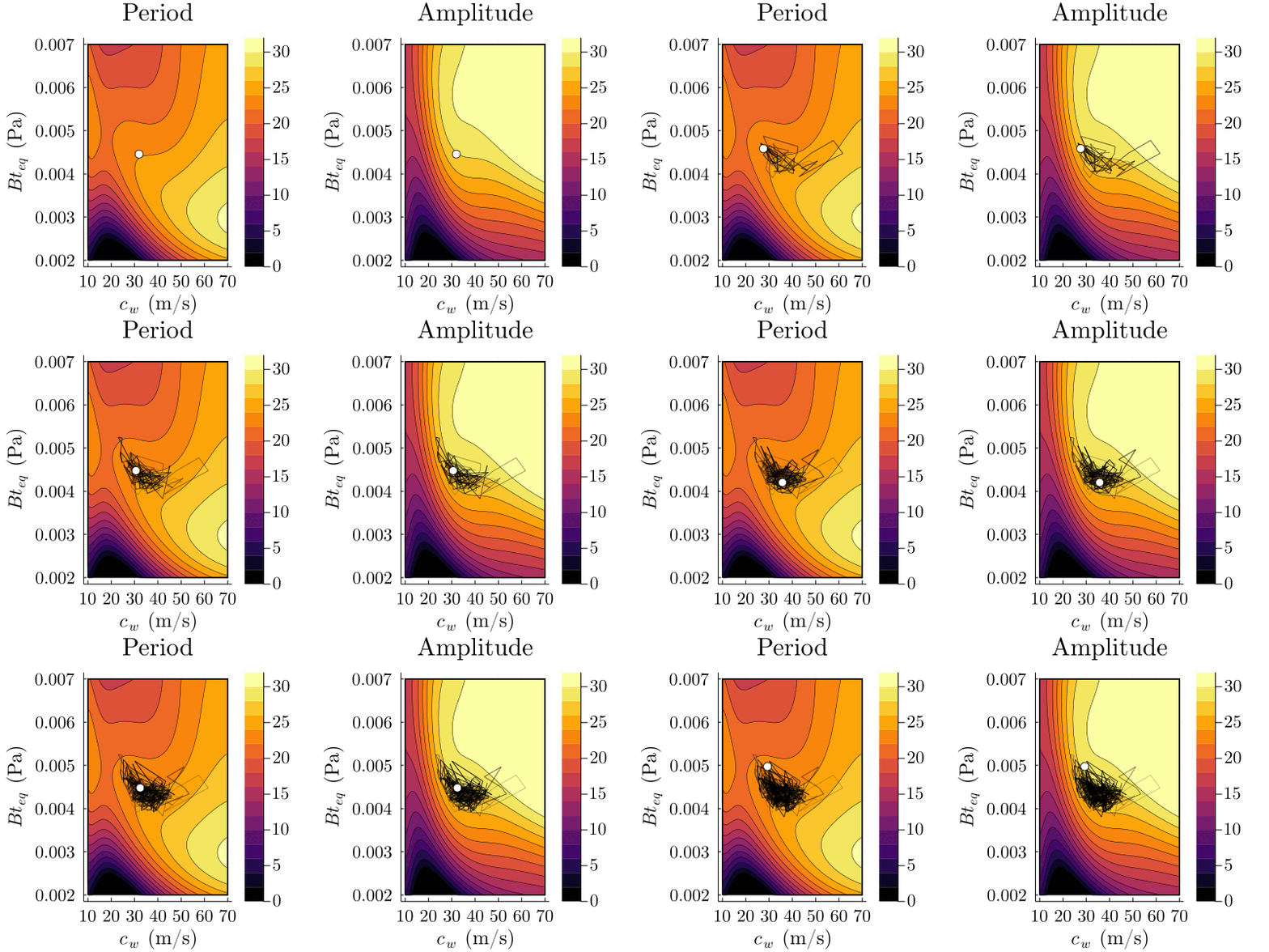
Next, we want to do uncertainty quantification, using Markov chain Monte Carlo (MCMC). We cannot regularly sample from the full climate model due to the high computational cost. However, using the ensembles of simulations generated in the calibration stage, we can build a Gaussian process emulator, which we can use for quick sampling. The figures below shows the behavior of the GP emulator with gravity wave parameters on the x- and y- axis for the QBO period (left) and amplitude (right). The points indicate MCMC samples, which are selected to be consistent with observations (including uncertainty).

The animation below shows how these samples generate a 2d posterior distribution of gravity wave parameters.